Sample description and DNA sequencing
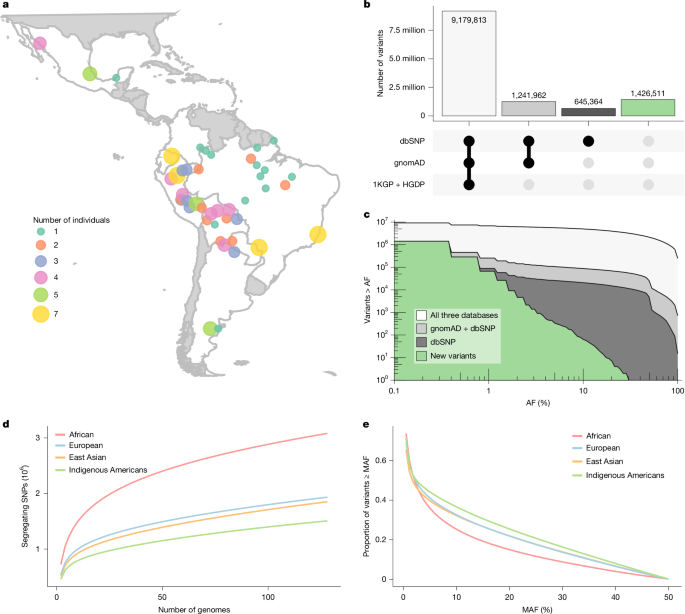
In this research, we generated new whole-genome sequencing (WGS) information from 128 Indigenous American people representing 45 populations and 28 language households throughout 8 Latin American nations (Extended Data Fig. 1 and Supplementary Note 1). Whole genomes had been sequenced on the Beijing Genomics Institute (China) and Dasa Genômica (Brazil) utilizing BGISEQ-500 and Illumina NovaSeq 6000, with a median sequencing depth of about 44×.
Ethical approval for pattern assortment was granted by native ethics committees in every nation: Argentina (Puerto Madryn Zonal Hospital, decision no. 009/2015; San Carlos de Bariloche Zonal Hospital, decision no. 1510/2015), Brazil (CONEP, decision nos. 763, 4599, 3828655, 7107656 and 8273857), Bolivia (Universidad Mayor de San Andrés), Ecuador (Universidad de Las Américas; Consejo Nacional de Ciencia y Tecnología—CONACyT, grant no. 69856; Instituto Nacional de Ciencias Médicas y de la Nutrición Salvador Zubirán, refs. 15,18), Mexico (CONACyT grant no. 69856; Instituto Nacional de Ciencias Médicas y de la Nutrición Salvador Zubirán, refs. 15,18; CNIC Salud 2013-01-201471; Committee of Ethics and Research, UADY, discover F-FENC-SAC-14/REV: 04, registry no. 09/17) and Peru (Universidad San Martín de Porres). Written knowledgeable consent was obtained from all individuals earlier than pattern assortment. Logistical assist in Brazil was supplied by the Fundação Nacional do Índio. All sampling adhered to the Declaration of Helsinki and the related nationwide legal guidelines and laws on the time (Supplementary Note 10).
Read mapping, variant calling and annotation
Whole-genome sequence information preprocessing, variant calling and annotation had been carried out utilizing the Sarek v.3.5.0 pipeline69. Specifically, sequence information in FASTQ format had been aligned to the GRCh38 reference genome and preprocessed in accordance with the GATK Best Practices for germline variant discovery and joint variant calling. Variants within the joint cohort variant name format had been then normalized and annotated utilizing the Ensembl Variant Effect Predictor (VEP)70 v.113, incorporating a number of annotation sources. Annotations from dbSNP, ClinVar and extra customized annotations had been retrieved utilizing SnpSift and VEP plugins. Ancestral alleles had been filtered utilizing the VEP Ancestral Allele plugin to enhance the specificity of downstream inhabitants genetic analyses. New SNVs had been recognized by evaluating their positions and alleles with these of the variants in public databases (1KGP18, HGDP13, gnomAD19 and dbSNP20). Variants absent from the dataset of greater than 270,000 people had been labeled as new (Supplementary Note 2).
Site frequency spectra
We estimated the quantity of segregating single-nucleotide polymorphisms (SNPs) as a operate of pattern measurement utilizing a rarefaction method on the premise of the positioning frequency spectrum (SFS). Alternate allele counts had been computed for biallelic websites and had been used to assemble the SFS utilizing Scikit-Allel v.1.3.13. To account for various pattern sizes and normalize the comparisons, the folded SFS was projected onto smaller pattern sizes utilizing a hypergeometric downsampling technique.
Dataset meeting and high quality management
Genomic coordinates of the newly sequenced people had been mapped to the hg38 reference genome. The 128 newly generated genomes had been merged with the next publicly accessible WGS databases (Supplementary Note 1): (1) 1KGP High Coverage, (2) HGDP and (3) SGDP. Sites and people with greater than 5% lacking information had been eradicated, biallelic SNVs had been chosen, and positions with important deviations (P < 10−8) from the Hardy–Weinberg equilibrium expectations had been excluded. Ambiguous positions (A-T and C-G) had been additionally eliminated. The ensuing dataset comprised 199 Indigenous American people from 31 language households and 53 ethnic teams. It contains 5,308,880 biallelic SNPs and 3,710 people from 201 populations worldwide.
After the preliminary high quality evaluation, linkage disequilibrium pruning was carried out with ‘SNPRelate’ v.1.28.0 R bundle71 to exclude markers exhibiting a pairwise correlation better than 20% (r2 > 0.2) in a 50-kb sliding window, advancing in 10-kb steps. This process yielded an linkage-disequilibrium-pruned dataset for downstream analyses that required an impartial set of markers (for instance, PCA and ADMIXTURE).
PCA
PCA was carried out utilizing the ‘SNPRelate’ v.1.28.0 R bundle71 on each the whole dataset and a subset comprising solely native ancestry-masked Indigenous American populations to evaluate potential biases launched throughout information merging and high quality management, in addition to to discover broad patterns of ancestry and genetic differentiation. In the case of the second evaluation, positions with greater than 10% lacking information had been eradicated, in addition to these with a minor allele frequency under 5%.
Global ancestry inference
We analysed the Indigenous American genomes utilizing the supervised mode of ADMIXTURE72 v.1.3.0 and three putative ancestry parts (Ok = 3) utilizing a reference panel of numerous African (Bantu from Kenya, Bantu from South Africa, Biaka, Dinka, Khomani-San, Mandenka, Mbuti, San and Yoruba), European (Basque, Bergamo Italian, French, Orcadian, Sardinian and Tuscan) and Indigenous American (Karitiana, Surui, Colombian and Pima) populations with out proof of current admixture with different continental teams, operating 10 impartial iterations with 100 bootstrap replicates per run. The consensus outcomes of impartial runs had been obtained utilizing CLUMPP73 v.1.1.2.
We additionally investigated the genetic construction of present-day Indigenous Americans and their relationship with historical Indigenous people via unsupervised ADMIXTURE analyses, contemplating 2 to 12 putative ancestry parts (Ok = 2 to Ok = 12) and visualized the outcomes utilizing PONG74 v.1.5. In the primary evaluation, we integrated a reference panel of African, European and East Asian populations to mannequin the non-Indigenous American ancestry. In the second evaluation, we masked non-Indigenous American ancestry (following the method detailed under) in present-day Indigenous American people and then mixed them with historical ones.
Relatedness evaluation and pattern choice
Subsequently, we carried out kinship evaluation to determine and take away intently associated people from the dataset, minimizing the bias launched by shut family members in downstream analyses. Using PLINK v.1.9 (ref. 75), we estimated the IBD between all pairs of people, calculated as PI_HAT = P(IBD = 2) + 0.5 × P(IBD = 1). On the premise of these estimates, we recognized the most important set of unrelated people by making use of a first-degree kinship cut-off. Filtering was performed utilizing PRIMUS76 v.1.9.0.
Haplotypic part, native ancestry inference and masking
The haplotypic part of the genomic information was statistically inferred utilizing ShapeIT4 (ref. 77) v.4.2.2, with the 1KGP dataset because the reference panel. The parameters had been adjusted for sequencing information utilizing the ‘–sequencing’ possibility, with the next settings: 15 burn-in iterations, 15 pruning iterations and 100 important iterations. Local ancestry inference was performed utilizing RFMix78 v.1.5.4, making use of a window measurement of 0.2 cM and a minimal of 5 reference haplotypes per tree node, utilizing a reference panel of unadmixed (that’s, with no proof of current admixture) Indigenous Americans, Sub-Saharan Africans and Western Europeans. We then used the inferred native ancestry tracts to masks genomic websites (code to carry out native ancestry masking is on the market at https://github.com/macscastro/lamask), assigning segments with a posterior chance of being ancestrally Indigenous Americans under 99% as lacking information (Supplementary Note 3).
Two additional datasets had been generated: (1) the primary dataset was generated by combining the native ancestry-masked dataset with ten Indigenous Andamanese, of which six had been Onge and 4 had been Jarawa79; and (2) the second dataset was created by combining the native ancestry-masked dataset with the Allen Ancient DNA Resource39 and historical DNA information from sambaqui mound builders present in Brazil15.
Effective migration floor modelling
EEMS modelling80 (https://github.com/dipetkov/eems) was utilized to subsets of 116 unadmixed and 160 ancestry-masked Indigenous Americans. The mannequin used 1,200 demes and ran for 4 × 10⁶ iterations with a 2 × 10⁵ burn-in interval (Supplementary Note 4). Migration and diversity charges had been visualized utilizing scripts from EEMS builders.
Patterns of allele sharing
Using the ‘admixtools’ v.2.0.10 R bundle, we calculated inhabitants pairwise f3(Mbuti; X, Y) to analyze genetic similarity patterns amongst modern Indigenous American populations. These patterns had been visualized utilizing a neighbour-joining tree and multidimensional scaling. The identical technique was used to evaluate spatial and temporal genetic variation, though genetic similarity was estimated for all pairs of modern and historical X and Y teams. Clusters with genetic similarities had been recognized as clades in a neighbour-joining tree. The 1 − outgroup f3 distances had been additionally used to deduce the existence of a correlation with geographic distances, estimated as nice circle distances with the R bundle ‘geosphere’ v.1.5.18.
Admixture graph and ancestry modelling
We used the ‘find_graphs’ operate from the ‘admixtools’ v.2.0.10 R bundle to determine believable inhabitants history fashions for modern Indigenous American populations (Supplementary Note 6). The algorithm ran ten occasions with 200 iterations for every inferred quantity of admixture occasions. The best-fitting admixture graph for every state of affairs (starting from zero to 5 admixture occasions) was chosen on the premise of its highest rating. These graphs had been constructed utilizing f2 statistics restricted to transversions, together with one consultant of every genetic cluster recognized within the earlier step.
To summarize our findings alongside present proof from the literature, we manually constructed admixture graphs and examined their match to the information utilizing the ‘qpgraph’ operate from ‘admixtools’ v.2.0.10 R bundle. Confidence intervals for drift lengths and admixture weights had been computed with the ‘qpgraph_resample_snps’ operate, which inserts the graph a number of occasions utilizing random SNP subsets. The outcomes had been summarized utilizing the ‘summarize_fits’ operate to generate a knowledge body with parameter estimates. As in earlier analyses, these fashions had been inferred utilizing solely transversions, thus avoiding systematic errors in historical DNA information brought on by postmortem harm, which induces C-to-T transitions at methylated CpG websites.
We used the qpWave technique to estimate the minimal quantity of impartial ancestral sources contributing to third-dispersal populations and the rotating qpAdm method to mannequin the sources and their proportional ancestry contributions to present-day Indigenous South Americans (Supplementary Note 6), each from the ‘admixtools’ v.2.0.10 R bundle. Analyses had been restricted to transversions with a most per-site lacking charge of 10%. Two complementary analyses had been carried out: (1) together with representatives from all genetic clusters and (2) specializing in people from the primary and second dispersals, alongside historical genomes from the North American Pacific Coast (that’s, excluding present-day Indigenous Americans and Ceramic-period Caribbeans). We recognized possible fashions through which supply contributions summed to 100% and plotted their possibilities and admixture proportions (Extended Data Fig. 11). Full mannequin statistics are reported in Supplementary Table 10.
Effective inhabitants measurement history and IBD sharing
We used IBDNe81 v.07May18.6a4 to deduce the efficient inhabitants measurement (Ne) histories of present-day Indigenous Americans. IBD segments had been recognized utilizing the Refined IBD82 v.12Jul18.a0b by merging these with brief gaps (most hole = 0.6, most discordant homozygotes = 1). Ne was inferred by pooling people by language households or genetic clusters (minimal ten people; populations from Mesoamerica and Aridoamerica had been pooled collectively), as earlier research point out that historic Ne trajectories stay strong with smaller pattern sizes (Supplementary Note 5). Segments better than 2 cM had been analysed utilizing the default IBDNe parameters.
IBD sharing patterns had been assessed by categorizing segments by size, which mirrored the time since a shared ancestor, to look at shared IBD inside and between populations over time. The IBD networks had been estimated utilizing the ‘as_tbl_graph’ operate (directed = FALSE) and visualized with the ‘ggraph’ operate (structure = ‘fr’) from the ‘tidygraph’ v.1.3.1 and ‘ggraph’ v.2.2.1 R packages, respectively.
Effective inhabitants measurement, coalescence charges and divergence occasions
We utilized the coalescent-based technique Relate83 v.1.2.2 to the phased WGS information to deduce historic modifications in Ne and estimate divergence occasions between modern populations. Input recordsdata had been transformed from variant name format to the haps/pattern format utilizing the RelateFileFormats script, and haplotypes had been flipped in accordance with the ancestral genome utilizing the Put togetherInputRecordsdata script, which additionally filtered SNPs and adjusted the distances on the premise of the genomic mappability masks. Input preparation was carried out utilizing the GRCh38 ancestral genome (human_ancestor_GRCh38), the GRCh38 genome masks (20160622_genome_mask_GRCh38) and GRCh38 recombination maps supplied by the developer.
Ancestral recombination graphs had been inferred utilizing the parameters −m = 1.25 × 10⁻⁸ (mutation charge) and −N = 30,000 (efficient inhabitants measurement), and the coalescence charge trajectories for every inhabitants had been estimated utilizing the EstimatePopulationSize script. Ne estimates had been obtained by calculating the inverted coalescence charge within the type of 0.5/(coalescence charge), and putative divergence occasions between teams had been recognized because the time factors at which the inverted coalescence charge values in every inhabitants began to diverge from each other, whereas the inverted cross-coalescence charge values between populations elevated. This signifies a lower in cross-coalescence charges between populations, indicating genetic separation and growing divergence over time. We additionally inferred the Ne history by inferring the ancestral recombination graph, whereas contemplating all people as a single inhabitants.
ROHs
ROHs had been inferred for unrelated and unadmixed Indigenous Americans utilizing PLINK v.1.9 with a sliding window of 50 SNPs, permitting for as much as one heterozygous web site and 5 lacking calls, a minimal density of one SNP per 50 kb, a most hole of 100 kb and a minimal ROH size of 500 kb. We in contrast the entire and common ROH lengths per particular person throughout international populations and Indigenous American clusters of genetic similarity. For international populations, we visualized particular person complete ROH counts and lengths, whereas for Indigenous Americans, we moreover plotted population-wise averages. We estimated the inbreeding coefficient (FROH − ROH-base inbreeding coefficient) and common inbreeding per inhabitants and examined the correlations between ROH counts and ancestry proportions. Additionally, ROH hotspots, outlined as areas with an above-average ROH prevalence (greater than three customary deviations), had been recognized (Supplementary Note 5).
Excess affinity with Australasian populations
We analysed the surplus genetic affinity between Indigenous American and Australasian populations by computing D(Mbuti, Australasian; X, Y), the place X and Y are Indigenous American teams, and Australasians are represented by Australian, Bougainville, Jarawa, Onge and Papuan (‘PapuanHighlands’ and ‘PapuanSepik’) populations. This included comparisons between present-day and historical Indigenous American populations to hint the Ypykuéra ancestry throughout area and time. To reduce bias from lacking information, we used a subset of unrelated and unadmixed Indigenous American people to make sure extra dependable outcomes when integrating present-day and historical genomes, the latter typically having excessive missingness ranges. We additionally investigated the signatures of pure choice in genomic areas with extra genetic affinity for Australasian populations (Ypykuéra ancestry) and their potential useful results (Supplementary Note 7).
Selection scans
Natural choice evaluation was carried out on a subset of unrelated people, masking segments of non-Indigenous American ancestry. To detect constructive choice indicators, we used two approaches primarily based on inhabitants differentiation (di statistic84 and PBS85) and prolonged haplotype homozygosity (iHS86 and xpEHH87). For all 4 statistics, we performed sliding-window evaluation utilizing 200 SNPs per window with a step measurement of 50 SNPs. We then mixed the genome-wide ranks of the 4 statistics for every window utilizing Fisher’s mixed rating88. This rating is calculated because the sum, over the 4 statistics, of −ln(rank of the statistic/quantity of home windows examined). Outlier areas had been outlined as home windows with Fisher’s mixed rating scores within the 99.ninth percentile (Supplementary Note 8).
Archaic introgression inference
To determine genomic areas exhibiting indicators of archaic introgression in ancestry-masked Indigenous Americans, we used segments detected by the SPrime technique89, utilizing Indigenous Americans as targets and African Mbuti from the HGDP as unadmixed outgroups. To improve robustness, we utilized filtering steps following ref. 64, retaining solely (1) high-confidence archaic websites and (2) these discovered at low frequency in Africa (lower than 0.01) however current at better than or equal to 0.01 in not less than one non-African inhabitants (Supplementary Note 9).
For websites passing via these filters, we labeled a match when the Archaic genotype contained the putative Archaic-specific allele (current in each Neanderthals and Denisovans). Additionally, we recognized Neanderthal-specific (matching Neanderthals however differing from Denisovans) and Denisovan-specific (matching Denisovans however differing from Neanderthals) websites.
ORA
ORA was carried out utilizing the WEB-based GEne SeT AnaLysis Toolkit (WEB-GESTALT)90, specializing in phenotypes and Gene Ontology classes, together with Biological Processes, Cellular Components and Molecular Functions. To deal with redundancy, we utilized a weighted set cowl method, which recognized the minimal subset of gene units that coated all genes from the enriched units. The weight or value of including a gene set was primarily based on P.
Reporting abstract
Further data on analysis design is on the market within the Nature Portfolio Reporting Summary linked to this text.